Previous   |    Next

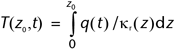
doi:10.2204/iodp.proc.304305.103.2006

Physical properties

The physical properties of basalt, diabase, gabbro, and peridotite cored at Site U1309 were characterized through a series of measurements on whole-core sections, split-core sections and pieces, and discrete samples as described in “Physical properties” in the “Methods” chapter. Natural gamma radiation (NGR) was not measured in Hole U1309B or between 40.5 and 131.1 mbsf in Hole U1309D because of a malfunction of the NGR data acquisition program.

Evaluation of physical properties at Site U1309 included nondestructive measurements of bulk density by gamma ray attenuation (GRA; for Hole U1309D core from >400 mbsf only), bulk magnetic susceptibility, noncontact resistivity (NCR), and NGR on whole cores using the MST as described in “Physical properties” in the “Methods” chapter. Sampling parameters for GRA, magnetic susceptibility, NCR, and NGR are summarized in Table T11 in the “Methods” chapter. Horizontal (x- and y-direction) and vertical (z-direction) P-wave velocities were measured on cubes, and they were measured in the x-direction only on minicores, cut from half-core samples. Porosity and bulk density were also determined from the cubes or minicores. Thermal conductivity was measured on polished half-core samples immersed in saltwater (and for Hole U1309D samples below 400 mbsf in an insulated box). Relatively high core recovery facilitated acquisition of an excellent physical properties data set.

Hole U1309B

Density and porosity

Measured values of bulk and grain density are summarized in Table T19 and Figure F256. Measured samples of basalt, diabase, and gabbro in this hole all have the same mean density, ~2.9 g/cm³, within their respective standard deviations of 0.05–0.08 g/cm³. The peridotite has a barely significantly lower density of 2.66 ± 0.08 g/cm³. The porosities are somewhat more variable, averaging 1.9% ± 1.4% for basalt, 2.1% ± 0.6% for diabase, 2.0% ± 0.8% for gabbro, 2.1% ± 1.6% for olivine and troctolitic gabbro, and 3.2% ± 0.3% for peridotite.

P-wave velocity is plotted against density in Figure F257. In this uppermost part of the section of the footwall at Site U1309, the points generally lie on the same linear trend as reported in the Leg 209 Initial Reports volume (Shipboard Scientific Party, 2004) for gabbro and peridotite data from Leg 153 (Cannat, Karson, Miller, et al., 1995) (Fig. F257).

Compressional wave velocity

Figure F256 shows the axial (x) component of compressional wave velocity plotted downhole with lithology indicated. We were not able to consistently measure velocity along the other two directions; where we did, uncertainties were relatively large and the velocities were not significantly different from the axial ones. The values are only moderately correlated with lithology (Figs. F257, F256). The average velocities for basalt and diabase are close (5.14 ± 0.33 km/s and 5.20 ± 0.27 km/s, respectively). The gabbros have slightly lower velocities, 4.99 ± 0.16 km/s, and olivine and troctolitic gabbros have slightly higher velocities of 5.54 ± 0.30 km/s. Peridotite velocity is significantly lower at 4.59 ± 0.12 km/s. The low velocity value for the peridotite reflects the high degree (60%–100%) of serpentinization observed in the samples and emphasizes the problem of identifying rock type from seismic velocity.

Thermal conductivity

Thermal conductivity was measured as described in “Physical properties” in the “Methods” chapter (Table T20). Measurements were made with the heating needle parallel and 35° to the core axis, and each run consisted of four measurements that were averaged for each data point. The standard deviation for these four measurements, averaged over all the Hole U1309B data points, is 0.08–0.09 W/(m·K), and only two data points (both in apparently isotropic basalts) had individual standard deviations >0.12 W/(m·K). The maximum difference between the 0°, +35°, and –35° measurements, also averaged over all the Hole U1309B data points, is 0.1 W/(m·K). We conclude that we are unable to detect any significant anisotropy of thermal conductivity within the precision of our measurements. We therefore averaged the three (or occasionally only one or two) directional measurements to yield each value reported in Table T19 and plotted in Figure F256.

Thermal conductivity is closely correlated with rock type in Hole 1309B (Table T20). Diabase shows the least thermal conductivity variation throughout the hole, whereas harzburgite has values of 3.7 ± 0.1 W/(m·K) and 4.1 ± 0.1 W/(m·K) measured at locations only 11 cm apart in the same piece. Alteration appeared in hand specimen to differ significantly between the two locations.

Magnetic susceptibility

Magnetic susceptibility was recorded on the MST. Measurements were taken every 2 cm on whole-round sections of core (Table T11 in the “Methods” chapter). The quality of these data tends to be degraded in RCB sections because the core is usually undersized with respect to liner diameter and is commonly disturbed by drilling. Volume susceptibility has therefore not been calculated, and all magnetic susceptibility data are presented in terms of IU (where 1 IU is on the order of 0.7 × 10^–5 SI). The lack of an exact relationship between IU and SI is due to fact that hard rock cores are not perfectly cylindrical and the diameter of individual pieces varies. Magnetic susceptibility is sensitive to variations in the type and concentration of magnetic grains in rocks and is thus an indicator of compositional variations and magnetic mineralogy. One major contribution to the magnetic susceptibility comes from ferro- and ferrimagnetic minerals such as magnetite, hematite, goethite, and titanomagnetite. Magnetic susceptibility can therefore be used to identify magnetite-rich zones, including oxide gabbros. Also, because magnetite is a by-product of serpentinization of olivine rich rocks, high magnetic susceptibility can indicate serpentinite intervals. Raw (i.e., unfiltered; see “Physical properties” in the “Methods” chapter) magnetic susceptibility amplitudes range from ~10 to >10,000 IU downhole (Fig. F256).

In Hole U1309B, susceptibility is related to rock type because of variations in concentration of magnetic minerals that vary with whole-rock composition. Figure F257 and subsequent plots show the MST measurements, made at 2 cm intervals along whole sections, in gray; “filtered” values, measured >5 cm from the ends of large pieces, are in red. Generally, the same trends are seen in both the 2 cm and the filtered data sets, although many low values measured near the ends of pieces have been removed. Occasionally, peaks in the 2 cm data have no corresponding value in the filtered data (i.e., were made near ends of pieces). An example is at 46.6 mbsf in Hole U1309D Unit 14, where the two highest points (7000–8000 IU) are missing from the edited data. Nevertheless, these removed data should not be ignored but simply recognized as being underestimates of the true values.

The highest susceptibility values measured in Hole U1309B are present in the serpentinite of Core 304-U1309B-11R, which has mean susceptibility of 5700 IU and maximum of ~9500 IU. The next highest values are in diabase, especially that of Core 304-U1309B-6R, Unit 22, and Cores 19R and 20R, Unit 62 (mean = 1800 IU; maximum = 6100 IU). The basalts generally have lower susceptibility (mean = 300 IU; maximum = 4600 IU). The lowest susceptibilities are located in the gabbros, with mean and maximum values of ~100 and 3000 IU, respectively. In fact, most gabbros have susceptibility <100 IU, with the following exceptions: short intervals of gabbro in Units 28 (Section 304-U1309B-9R-2, 49.84 mbsf) and 31 (Section 304-U1309B-10R-1, 53.46 and 53.82 mbsf) have susceptibility peaks of up to 300 IU. Unit 50 shows a more substantial increase, though again over a short interval, to just over 1000 IU in Section 304-U1309B-16R-2 at 82.49 mbsf. Aside from these intervals, the gabbros in Hole U1309B have uniformly very low magnetic susceptibility.

Most of the basalt and diabase have relatively uniform susceptibilities within each unit, but a few diabase units show marked transitions from one fairly uniform (and commonly very low) level to another within what is petrologically described as the same lithologic unit. Such transitions are listed in Table T21 and illustrated in Figure F258.

These variations in susceptibility reflect the proportion of magnetic minerals present (primarily magnetite; see “Paleomagnetism”) that may result either from variations in chemical composition or in subsequent alteration. In some instances, particularly in Unit 20, and on a larger scale in Unit 62, there is a symmetric pattern of moderate susceptibility at the unit margins (sometimes recognized by finer grain size) and much lower susceptibility in the interior, suggesting possible influence of emplacement mechanism (e.g., emplacement of multiple sheets with cryptic boundaries or flow-banding). The harzburgite (Unit 32) also displays some internal variability (Section 304-U1309B-11R-2 [e.g., ~58.89 mbsf]).

Electrical resistivity

The trends of the electrical conductivity and susceptibility curves are quite similar (Fig. F256). This suggests that the same minerals are responsible for both the magnetic susceptibility and the electrical conductivity. The mineral primarily responsible for the susceptibility is probably magnetite, which has the highest susceptibility of all minerals (6.0 SI) (Telford et al., 1976; Blum, 1997, quoting Thompson and Oldfield, 1986) and has been documented in many of the rocks from Hole U1309B. Magnetite can also be strongly electrically conductive compared to silicates, with a mean conductivity in the range 2 × 10^–4 to 2 × 10⁴ Siemens/m (S/m) (Telford et al., 1976). Ilmenite may also contribute; it tends to occur with magnetite in basalt and diabase, though not in serpentinite, and has susceptibility of 2.0 SI and conductivity of 0.02 to 10³ S/m. Pyrrhotite and pyrite, though magnetic and electrically conductive, might contribute in places but are not pervasively present in the rock recovered in Hole U1309B.

Hole U1309D

Density and porosity

Bulk density, grain density, and porosity in Hole U1309D (Fig. F259; Table T22) were calculated from the wet mass, dry mass, and dry volume of discrete rock cubes using moisture and density method C for igneous rocks (see “Physical properties” in the “Methods” chapter) in Cores 304-U1309D-1R through 78R and 305-U1309D-80R through 295R (20.5–1415.3 mbsf). Although GRA density was acquired on some whole-round sections of core (with a sampling rate of 2 cm) (Table T11 in the “Methods” chapter), these data should not be used for analytical applications; they are consistently too low because the RCB core did not fill the core liner and the core was commonly broken. GRA density has an important practical application in that rapid decreases in this parameter can be used to map the location of breaks along the core. The moisture and bulk density data are substantially more accurate, and we use these data in describing the downhole density variations.

Bulk density is a measure of the bulk weight divided by the sample volume. To introduce some redundancy into the measurement process (in case of problems with the pycnometers), the wet volume was also estimated using a caliper to measure the cube dimensions (which we refer to as method D). This and method C should give similar values. A plot of bulk density by caliper versus bulk density by pycnometer gives an error of –0.018 ± 0.0007 g/cm³ (Fig. F260). Although both methods accurately represent bulk density, we continue to use the moisture and density–calculated bulk density for description. The caliper-calculated bulk density is more inaccurate with cubes that have nonparallel sides or are chipped, as demonstrated, for example, by a cube that plots around 3.3 g/cm³ (caliper) and 3.45 g/cm³ (pycnometer) and whose corners were chipped because of the fractured nature of the source material.

For the combined Expedition 304 and 305 data, bulk density varies between 2.45 and 3.56 g/cm³ (Fig. F259B). There is a general slight increase in density downhole from 0 to 1100 mbsf, after which the scatter increases significantly. Below 1230 mbsf, the density is constant or slightly decreasing to the bottom of the hole. High densities correlate with fresh oxide gabbros and olivine-rich troctolites. Bulk density scatter tends to decrease with depth, except for a notable increase in scatter between 1100 and 1230 mbsf associated with the presence of olivine-rich troctolites. There is no obvious and consistent correlation with rock type. The increased bulk density scatter within the 1100–1230 mbsf interval relates to the alternation of relatively lower density gabbros with higher density olivine-rich assemblages.

Porosity reflects a combination of crystal fabric, stress history, volume changes induced by metamorphic alteration, vertical unloading, and cracking of the rocks during drilling. Porosity is calculated from the volume of pore water, assuming complete saturation of the rocks (Blum, 1997) (see “Physical properties” in the “Methods” chapter). For the combined Expedition 304 and 305 data, the porosity ranges between 0.0% and 6.4% with a mean of 1.1% ± 0.94% (Fig. F259D). Porosity and bulk density vary similarly downhole, showing a change from increased scatter and porosities generally 1%–2.5% in the upper part of Hole U1309D to significantly reduced scatter and decrease from ~700 mbsf to the bottom of the hole. The discrete zones of relatively high porosities and low bulk densities at 30–85, 420–450, 560–575, 635–645, 685–700, and 1095–1135 mbsf correlate with zones of cataclastic deformation and fault zones (see “Structural geology”).

Compressional wave velocity

Compressional wave velocities were measured at 1 atm with the P-wave sensor (PWS3) contact probe system on minicores for depths <400 mbsf (Expedition 304) and ~10 cm³ rock cubes for greater depths (Expedition 305). Velocity was measured along axis of the minicores (x-direction), whereas the cubes were used to measure velocities in the horizontal (x- and y-) and vertical (z-) directions. Apparent seismic anisotropy was calculated from the measured velocities of the cubes (Fig. F261). A test was performed to evaluate the precision of velocity measurements using the PWS3 Hamilton Frame. Sample 305-U1309D-107R-4, 48–50 cm, was measured ~80 times in the x-direction, and a running average was calculated (Fig. F262). Eventually, after ~50 measurements, the running mean converged to a value of 6.07 km/s, although the rate of convergence may have been slowed because of the progressive drying of the cube during the experiment. (The small kink at 72 measurements marks the rewetting and retightening of the caliper at this point). These statistics suggest a measurement error of <1%. It is recommended that the acquisition program be modified to average 20–40 values rather than relying on a single value.

Downhole variations in velocity (Fig. F263) are scattered in the upper 150 m of Hole U1309D, show a slight decrease from ~150 to 350 mbsf, and increase between 350 and 450 mbsf. This is followed by another generally constant value from 400 to 800 mbsf, after which there is a steady decrease in velocity to the bottom of the hole. The velocities between 20 and 350 mbsf average ~5.5 km/s, and those between 600 and 800 mbsf average ~6.0 km/s, whereas the velocities between 1200 and 1400 mbsf show a decreasing trend and an average of ~5.5 m/s. Density is either constant or slightly increasing over the same interval, so no definite conclusions can be made without further work. Velocities measured along the x-axis in the minicores range from 4.0 km/s (in serpentinized peridotite) to 6.2 km/s in olivine gabbro. Velocity of the rock cubes from Hole U1309D range between 4.65 and 6.83, 4.81 and 6.77, and 4.80 and 6.67 km/s in the x-, y-, and z-directions, respectively (Fig. F261).

Superimposed on the long-wavelength velocity trend are a number of smaller, local variations. Downhole variations are not simply related to rock type (Fig. F263). Abrupt velocity variations occur at 325, 440, 468, 547, 584, 642, 690, 810, 942, 1000, 1190, 1251, and 1362 mbsf. The largest velocity variations are located between 350 and 450 (an increase), 600 and 650 (a decrease), and 920 and 950 mbsf (a decrease) and are associated with intervals of massive olivine gabbro and troctolitic gabbro. Despite these local associations of velocity variation with lithology, the bulk of the measurements are not simply related to rock type, including the olivine-rich troctolite, but also to alteration and/or deformation.

The x-y velocity anisotropy ranges between –9% and 14% with an average not statistically different than zero (Fig. F261). There does not appear to be any systematic variation with x-y anisotropy with depth, although the scatter increases significantly between 1000 and 1200 mbsf. In contrast, the vertical-horizontal velocity anisotropy ranges principally between –6% and 11%. There appears to be a systematic variation in the vertical-horizontal anisotropy from a zero or slightly negative value between 400 and 700 mbsf, changing to a few percent positive anisotropy from 750 to 1000 mbsf. Below this, the scatter increases significantly (Fig. F261), probably as a consequence of strong variations in alteration in the olivine-rich troctolite and associated gabbros (see “Metamorphic petrology”).

The relationship between P-wave seismic velocity and bulk density measured during Expeditions 304 and 305 is compared to results from Leg 209 in Figure F264. A large amount of highly serpentinized peridotite was recovered during Leg 209, which explains the spread to lower density and velocity values compared to Hole U1309D samples. A significant subset of gabbro and diabase samples from Leg 209 show higher densities for a given velocity. This is related to the occurrence of abundant Fe-Ti oxides in numerous 209 samples (Shipboard Scientific Party, 2004). Hole U1309D data also follow a trend similar to gabbro and peridotite recovered in the MARK area during Leg 153 (see Fig. F88 in Shipboard Scientific Party, 2004), although they are more scattered, likely reflecting the wider spectrum of primary lithology and alteration.

Changes in velocity do not show any systematic correlation with trends from other Expedition 304 and 305 igneous, metamorphic, or structural data sets, including alteration, modal olivine content, or Fe₂O₃ variation. Figure F265 explores the relationships between Expedition 304 and 305 PWS velocities (z-velocity), logging velocities, porosity, and fracture intensity (see “Structural geology” for details on calculating fracture frequency). Between 0 and 350 mbsf, the logging velocities, which approximate an in situ velocity estimate, are systemically lower than the measured PWS velocities. Over this same depth range, moisture and density porosities range from 1% to 6%, reaching a local minimum at ~400 mbsf. The qualitative fracture frequency distribution, similar in scale to the PWS and moisture and density data estimates, likewise shows that the degree of macroscopic fracturing is a maximum in the upper part of the section and systematically decreases to 380–400 mbsf (Fig. F265). Between 400 and 800 mbsf, the PWS and logging velocities are coincident. Below 800 mbsf, there is a hint of the logging velocities increasing relative to the PWS velocities, but the lack of deeper logging data (see “Downhole measurements”) makes it impossible to know if the trend is real or just local variability. Porosity is a minimum between 800 and 1200 mbsf. Fracture frequency falls rapidly to values mostly <0.5 below 800 mbsf, following a trend similar to porosity which averages 0.6% for this lower portion of the core.

The interrelationship between logging and PWS velocity, porosity, and degree of fracturing suggests that the velocity behavior with depth is primarily a function of the reduction in opening of fractures and microcracks that is related to increasing overburden pressure. The pattern in the upper ~220 m can be explained by fewer open/visible fractures, consistent with the fracture intensity and porosity variability (given that the fractured, and thus higher porosity, rocks are unlikely to be sampled by drilling). Between 600 and 800 mbsf, the reduction in the amount of open microcracks is suggested by the coincidence of logging and PWS velocities. Below ~800 mbsf, we expect a systematic decrease in rock volume determined by Poisson’s ratio and overburden stress. Without a continuous sonic data set from the lowermost 600 m of Hole U1309D, it is impossible to test this hypothesis or to determine if the measured cube velocities (not measured at in situ pressures) are accurately representing the velocity deeper in the hole.

Thermal conductivity

Thermal conductivity measurements were done on intact pieces of archive-half core at least 10 cm in length (Table T23). Silicon carbide powder (120 grit) was used to polish most rocks from Expedition 304 and all rocks from Expedition 305 prior to their being measured for thermal conductivity, which, coupled with isolating the experiment from drafts, significantly increased the precision of the measurements. Because the majority of the rocks did not show preferred fabric or crystal alignments, and based on the conclusion of Expedition 304 experiments, no attempt was made to measure thermal conductivity anisotropy.

Measured thermal conductivity in Hole U1309D rocks ranges between 1.71 and 4.34 W/(m·K), with an average value of 2.43 ± 0.45 W/(m·K) (Fig. F266). There is an overall decrease in the scatter of the thermal conductivity measurements with depth between seafloor and 1100 mbsf, primarily reflecting the reduction in igneous rock lithologic variability with depth (see “Igneous petrology”). The thermal conductivities show a subtle relationship with lithology. In particular, the olivine-rich troctolites have consistently high thermal conductivities. Average values for all measurements in Hole U1309D are given in Table T22 (Fig. F266).

Temperature

Because the oceanic crust of Atlantis Massif is young (1.5–2 Ma), there was a concern that maximum temperatures at depths of 800–1400 mbsf might damage the downhole logging tools. Attempts to measure ambient bottom hole temperatures proved to be difficult because of a malfunctioning Water Sampling Temperature Probe (WSTP). Furthermore, flushing of the bottom of the hole with cold surface waters during drilling meant that any temperature measurement would necessarily be a minimum. A set of "thermal tabs" was placed around the core catcher during a dedicated (noncoring) core barrel run (see “Operations”). These simple devices measure the maximum bottom hole temperature by registering a color change in the tab. To test and calibrate this device, a thermal tab was placed in the Physical Properties oven, which is kept at a constant 105° ± 5°C. Figure F267 shows the before and after color state of the thermal tab. The color change indicates that the maximum temperature experienced by the tab was between 98° and 104°C, consistent with its rating. These thermal tabs were used to estimate minimum bottom hole temperatures when deployed.

Figure F268 shows the results of modeling crustal temperatures in Hole U1309D. Theoretical temperatures versus depth curves were generated using basal heat fluxes of 226 and 206 mW/m², consistent with oceanic crust of 1 and 2 Ma, respectively, for a cooling plate model (thick red and blue lines, Fig. F268). The age range was selected to approximate the conductive temperature distribution of the crust (neglecting any effects of hydrothermal fluid circulation in the crust). The temperature structure at the spreading center was assumed to be consistent with a 5 km crust and a 14.5 km thick lithosphere. The anomalous basal heat flow, q(t), is calculated by assuming a lithosphere of 125 km at thermal equilibrium (i.e., a linear geothermal gradient between the surface at 5°C and an asthenosphere temperature of 1333°C) and crustal thickness of 31.2 km; crustal and mantle extension factors of 6.24 and 10, respectively, mimic the structure and thermal state of young oceanic lithosphere.

Fourier’s law was then used to calculate the temperature as a function of depth for the range in basal heat flows and the observed thermal conductivity distribution in Hole1309D (Fig. F266):

where T(z_o ,t) is the rock temperature as a function of depth, z_o , and time t since the initiation of cooling, and κ_r(z) is the measured thermal conductivity structure of the basement rocks.

Maximum estimated temperature (disregarding cooling effects by water circulation during drilling) at the base of Hole U309D is ~142°C. Measured temperatures are offered by three methods (Fig. F268):

1. Thermal tabs, giving a minimum temperature of 70° and 108°C at 1171 and 1220 mbsf (red circles), respectively.
2. Temperature estimates from the downhole logging tool (triple combination [triple combo] TAP tool; 52°C at 562 mbsf, 57°C at 700 mbsf, and 69°C at 754 mbsf; yellow circles).
3. From the Goettingen Borehole Magnetometer (GBM), which monitors temperature as a function of time both during descent (purple curve) and ascent (pink curve) of the tool.

It is concluded that a conductive gradient generally characterizes the temperature structure of the hole, at least in the upper ~1 km (see “Downhole measurements”) now modified by drilling water circulation, and that maximum temperature may be in the range of 130°–145°C.

Magnetic susceptibility

As in Hole U1309B, magnetic susceptibility is related to lithology because of the occurrence of magnetic minerals being more common in certain rock types than others (Fig. F269).

The basalts in the upper section of Hole U1309D have low susceptibility. Diabase units have high susceptibility intervals. Figure F270 shows the variation of susceptibility along each of the major diabase units (Units 1, 12, 14, and 44; see “Igneous petrology”). The pattern of variation itself is quite variable: in Unit 1, moderate peaks straddle a 1 m thickness with very low susceptibility, in large parts of Units 12 and 44, susceptibility increases fairly steadily downcore, and in Unit 14, it decreases downcore. However, there are more local variations; for example, in a single 30 cm long piece at 44.5 mbsf (Section 304-U1309D-6R-3 [Piece 3]), susceptibility increases 16-fold from 350 to 5770 IU within a 20 cm interval. These variations in magnetic susceptibility do not correlate with any of the changes noted in the lithologic descriptions. Although variations in grain size up- or downcore or from unit center to edges have been noted, usually magnetic susceptibility is invariant to changes in grain size. It is likely that the observed susceptibility changes reflect both varying magnetic mineral content (Fig. F271) and varying degrees of alteration of magnetite (Fig. F272).

The highest susceptibilities measured in Hole U1309D were in the oxide gabbro units. In several intervals, values exceed the maximum range of the sensor. However, in some intervals, a relatively simple signal and moderate downhole susceptibility gradient allow the full signal to be reconstructed by adding multiples of 10,000 IU to the logged value, and the required multiple can be verified by using the excellent correlation between electrical conductivity and susceptibility (Fig. F273). Performing such an adjustment to the logged susceptibility from the oxide gabbros in Hole U1309D Cores 304-U1309D-35R and 36R shows that the true susceptibility probably peaks at 24,700 IU at 193.08 mbsf (Fig. F274). If all the susceptibility is carried in magnetite, this requires a volume fraction of 8% magnetite. Other oxide gabbros also have high and variable measured susceptibility values, suggesting true susceptibilities >10,000 IU in places, although we have not attempted to adjust other parts of the data. As with the other rock types cored in Hole U1309D, the susceptibility in the oxide gabbros can vary significantly within a single unit.

Gabbros (including olivine- and orthopyroxene-bearing gabbros) in Hole U1309D mostly have low susceptibility (<500 IU), although there are local decimeter-scale bands of higher susceptibility. Olivine and troctolitic gabbros in Hole U1309D mostly have low susceptibility (<500 IU). However, there are local bands of higher susceptibility with peaks up to 7500 IU. Troctolites carry low to moderate susceptibility.

Ultramafic rocks (olivine-rich troctolite, dunite, and harzburgite) in Hole U1309D can have very high susceptibilities, with a maximum of 12,100 IU estimated at 173.12 mbsf by adjusting the logged values as described above. These high values are associated with intervals that are highly serpentinized.

A feature of the susceptibility values recorded from the mafic and ultramafic rocks at Site U1309 is the extreme variability over a short vertical distance. In Hole U1309D, this is well exemplified in Units 147–163 (310–328 mbsf; Fig. F275). The very high values 321–322 mbsf reach and may locally exceed the maximum recording level of 10,000 IU, compared to very low values near the top and bottom of the unit. Many detailed correlations between susceptibility change and lithologic boundaries can be seen in this interval. The detailed variations in susceptibility patterns also provide a possible means of stratigraphic correlation. For example, the correlation between the diabase units in Hole U1309B, 94–101 mbsf, and Hole U1309D, 85–94 mbsf, and that between the diabase unit in Hole U1309B, 62–78 mbsf, and the one in Hole U1309D, 43–48 mbsf, are based on the similarity of the magnetic susceptibility pattern along each pair of units (see “Correlations between Holes U1309B and U1309D”).

Extreme magnetic susceptibility amplitudes correlate with zones of serpentinization (and the production of magnetite), oxide- and sulfide-bearing gabbros, and troctolites and olivine-rich troctolites. There is, therefore, an excellent relationship between magnetic susceptibility and those lithologies rich in ferro- and ferrimagnetic minerals.

Electrical resistivity

Noncontact resistivity was derived from voltages measured on the MST. Measurements were taken every 2 cm on whole-round sections of core (Table T11 in the “Methods” chapter). NCR measurements, in volts (and as stored in the IODP database), were converted to resistivity using the calibration done during Expedition 304 (see notes on limitations of NCR data in “Physical properties” in the “Methods” chapter). The reciprocal of electrical resistivity (NCR) is electrical conductivity (NCC) with units of S/m. The magnetic susceptibility, NCR, and NCC data tend to be highly variable, so, to see the general variation and interrelationships, the data have been filtered using a 51-point running average (Fig. F276). A caution, however: some of the extreme magnetic susceptibility variations are a function of the 10,000 IU wrap-around problem documented in “Physical properties” in the “Methods” chapter. Nevertheless, a strong correlation exists between conductivity and magnetic susceptibility (Fig. F276). This suggests that the same minerals are responsible for both the magnetic susceptibility (high magnetic susceptibility) and the electrical conductivity (high NCC). Likely candidates are oxides and sulfides. The primary mechanism for noncontact electrical conductivity here is likely to be electronic via conducting minerals (oxides and sulfides), rather than ionic through pore fluids (especially seawater).

We attempted to test whether high NCR values reflected an electronic source versus an ionic source on two large pieces of olivine-bearing gabbro—Section 304-U1309D-57R-1 (Pieces 6 and 7)—by measuring resistivity on the MST following saturation for different times in seawater (Fig. F277). Measurements (at atmospheric pressure) were made on nominally dry rock (following curation in the Core Laboratory for several days) and then after the indicated periods of saturation in seawater. No significant variation was observed up to 34 h of saturation, implying that ionic conduction is not an important mechanism in these samples. This is probably due to a combination of low porosity and high volume percent of conducting minerals.

Three main magnetic susceptibility and NCC responses are recognized (Fig. F276):

1. Very low magnetic susceptibility and NCC amplitudes (0–500 IU and less than ~0.1 mS/m, respectively) associated with diabase, coarse- and medium-grained gabbros, and locally very fresh olivine-rich troctolite;
2. Intermediate amplitudes (1000–2000 IU and ~0.2–0.4 mS/m) associated with olivine gabbros; and
3. Extreme amplitudes (6,000–10,000 IU and less than ~1.5 mS/m) associated with oxide gabbros and serpentinized troctolites (Fig. F276).

Although variations in grain size up- or downcore have been noted, usually susceptibility is invariant to changes in major lithologic grain size. It is likely that the observed susceptibility changes reflect a combination of varying Fe content, magnetite/ilmenite ratio, and degrees of alteration. More than 90% of the magnetic susceptibility values are between 0 and 2000 IU (with corresponding NCC values of ~0–0.5 mS/m), which is associated with the various nuances of gabbroic compositions observed in the core (coarse-, medium-, and fine-grained gabbro, olivine gabbros, olivine-bearing olivines, amphibole-bearing olivines, gabbronorite gabbros, etc.). Even larger olivine-rich troctolite intervals (669.5–671.5 and 1100–1250 mbsf) are not always associated with significant and unambiguous magnetic susceptibility and NCC amplitudes. Small-scale variations relate to variable degrees of serpentinization.

The location of most of the major oxide gabbros and troctolites are obvious from the magnetic susceptibility/NCC signals (Fig. F276). In contrast, the opposite extreme is represented by rocks between 460 and 491 mbsf and 731 and 772 mbsf, which are characterized by extremely low magnetic susceptibility and NCC signatures. These regions consist of coarse-grained gabbro, olivine gabbro, diabase, and olivine-bearing gabbro. In marked contrast, the same rock types can also be associated with relatively high magnetic susceptibility and NCC values, such as the regions between 780 and 800 mbsf and 856 and 862 mbsf (in this case, massive gabbros).

Natural gamma radiation

The variations of natural gamma ray counts along the core are shown in Figure F278. Measurements were taken every 10 cm on whole-round sections of core with a 30 s sampling period (Table T11 in the “Methods” chapter). The relatively large sampling interval was selected because a low NGR was expected; the low-resolution acquisition rate was simply to monitor NGR amplitude and trend to help with calibration of the logging tools. As seen in Figure F278, the NGR response is not significantly different from the background level.

Conclusions

• Susceptibility shows a general increase with magnetic mineral content, consistent with the conclusion that it is mostly carried in iron-rich oxides, probably mainly magnetite.
• Alteration often contributes to the decreased susceptibility in diabase (magnetite converted to ilmenite) and increased susceptibility in olivine-rich lithologies (production of magnetite during serpentinization).
• Highest susceptibility (>10,000 IU) is frequently present in oxide gabbros; ultramafic rocks generally have high susceptibility (approximately <10,000 IU), probably carried in magnetite produced by serpentinization; basalts and diabases have variable to high susceptibility; gabbros generally have very low susceptibility, but with some moderate- to high-susceptibility zones—the latter perhaps reflecting higher olivine/serpentine content.
• High susceptibility is not present uniformly through lithologic units but tends to concentrate in zones and narrow bands—often near tops or bottoms of units.
• Magnetic susceptibility and electrical conductivity are highly correlated, implying that the same minerals carry each signal.
• Electrical conductivity is not strongly dependent on water saturation, implying that conduction is mostly electronic (in oxide or possibly sulfide minerals), not ionic (in pore water).
• Thermal conductivity is generally highest and most variable in peridotites and olivine-rich troctolites. Gabbros generally have thermal conductivity of 2.0–3.0 W/(m·K). Olivine and troctolitic gabbros can range to higher values similar to the ultramafic rocks (3.0–3.5 W/[m·K]). Basalts and diabases consistently have lower conductivity (generally 2.0–2.3 W/[m·K]).
• P-wave velocity is most variable (4.0–5.7 km/s) in ultramafic rocks, presumably dependent on degree of serpentinization.
• P-wave velocity and density show no simple relation to rock type.
• P-wave velocity variation with depth probably reflects reduced opening of fractures and microfractures with increasing overburden, but our sample measurements do not show a simple monotonic or step increase.
• NGR shows no significant anomalies.

Top of page   |    Previous   |    Next